Geonames in CubicWeb !
CubicWeb is a semantic web framework written in Python that has been succesfully used in large-scale projects, such as data.bnf.fr (French National Library's opendata) or Collections des musées de Haute-Normandie (museums of Haute-Normandie).
CubicWeb provides a high-level query language, called RQL, operating over a relational database (PostgreSQL in our case), and allows to quickly instantiate an entity-relationship data-model. By separating in two distinct steps the query and the display of data, it provides powerful means for data retrieval and processing.
In this blog, we will demonstrate some of these capabilities on the Geonames data.
Geonames
Geonames is an open-source compilation of geographical data from various sources:
"...The GeoNames geographical database covers all countries and contains over eight million placenames that are available for download free of charge..." (http://www.geonames.org)
The data is available as a dump containing different CSV files:
- allCountries: main file containing information about 8,000,000 places in the world. We won't detail the various attributes of each location, but we will focus on some important properties, such as population and elevation. Moreover, admin_code_1 and admin_code_2 will be used to link the different locations to the corresponding AdministrativeRegion, and feature_code will be used to link the data to the corresponding type.
- admin1CodesASCII.txt and admin2Codes.txt detail the different administrative regions, that are parts of the world such as region (Ile-de-France), department (Department of Yvelines), US counties...
- featureCodes.txt details the different types of location that may be found in the data, such as forest(s), first-order administrative division, aqueduct, research institute, ...
- timeZones.txt, countryInfo.txt, iso-languagecodes.txt are additional files prodividing information about timezones, countries and languages. They will be included in our CubicWeb database but won't be explained in more details here.
The Geonames website also provides some ways to browse the data: by Countries, by Largest Cities, by Highest mountains, by postal codes, etc. We will see that CubicWeb could be used to automatically create such ways of browsing data while allowing far deeper queries. There are two main challenges when dealing with such data:
- the number of entries: with 8,000,000 placenames, we have to use efficient tools for storing and querying them.
- the structure of the data: the different types of entries are separated in different files, but should be merged for efficient queries (i.e. we have to rebuild the different links between entities, e.g Location to Country or Location to AdministrativeRegion).
Data model
With CubicWeb, the data model of the application is written in Python. It defines different entity classes with their attributes, as well as the relationships between the different entity classes. Here is a sample of the schema.py that we have used for Geonames data:
class Location(EntityType):
    name = String(maxsize=1024, indexed=True)
    uri = String(unique=True, indexed=True)
    geonameid = Int(indexed=True)
    latitude = Float(indexed=True)
    longitude = Float(indexed=True)
    feature_code = SubjectRelation('FeatureCode', cardinality='?*', inlined=True)
    country = SubjectRelation('Country', cardinality='?*', inlined=True)
    main_administrative_region = SubjectRelation('AdministrativeRegion',
                              cardinality='?*', inlined=True)
    timezone = SubjectRelation('TimeZone', cardinality='?*', inlined=True)
    ...
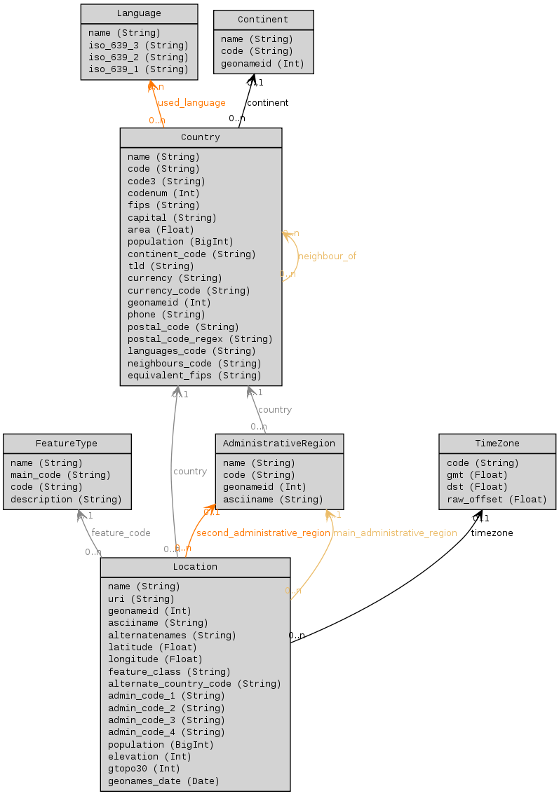
This indicates that the main Location class has a name attribute (string), an uri (string), a geonameid (integer), a latitude and a longitude (both floats), and some relation to other entity classes such as FeatureCode (the relation is named feature_code), Country (the relation is named country), or AdministrativeRegion called main_administrative_region.
The cardinality of each relation is classically defined in a similar way as RDBMS, where * means any number, ? means zero or one and 1 means one and only one.
We give below a visualisation of the schema (obtained using the /schema relative url)
Import
The data contained in the CSV files could be pushed and stored without any processing, but it is interesting to reconstruct the relations that may exist between different entities and entity classes, so that queries will be easier and faster.
Executing the import procedure took us 80 minutes on regular hardware, which seems very reasonable given the amount of data (~7,000,000 entities, 920MB for the allCountries.txt file), and the fact that we are also constructing many indexes (on attributes or on relations) to improve the queries. This import procedure uses some low-level SQL commands to load the data into the underlying relational database.
Queries and views
As stated before, queries are performed in CubicWeb using RQL (Relational Query Language), which is similar to SPARQL, but with a syntax that is closer to SQL. This language may be used to query directly the concepts while abstracting the physical structure of the underlying database. For example, one can use the following request:
Any X LIMIT 10 WHERE X is Location, X population > 1000000,
    X country C, C name "France"
that means:
Give me 10 locations that have a population greater than 1000000, and that are in a country named "France"
The corresponding SQL query is:
SELECT _X.cw_eid FROM cw_Country AS _C, cw_Location AS _X
WHERE _X.cw_population>1000000
      AND _X.cw_country=_C.cw_eid AND _C.cw_name="France"
LIMIT 10
We can see that RQL is higher-level than SQL and abstracts the details of the tables and the joins.
A query returns a result set (a list of results), that can be displayed using views. A main feature of CubicWeb is to separate the two steps of querying the data and displaying the results. One can query some data and visualize the results in the standard web framework, download them in different formats (JSON, RDF, CSV,...), or display them in some specific view developed in Python.
In particular, we will use the mapstraction.map which is based on the Mapstraction and the OpenLayers libraries to display information on maps using data from OpenStreetMap. This mapstraction.map view uses a feature of CubicWeb called adapter. An adapter adapts a class of entity to some interface, hence views can rely on interfaces instead of types and be able to display entities with different attributes and relations. In our case, the IGeocodableAdapter returns a latitude and a longitude for a given class of entity (here, the mapping is trivial, but there are more complex cases... :) ):
class IGeocodableAdapter(EntityAdapter):
      __regid__ = 'IGeocodable'
      __select__ = is_instance('Location')
      @property
      def latitude(self):
          return self.entity.latitude
      @property
      def longitude(self):
          return self.entity.longitude
We will give some results of queries and views later. It is important to notice that the following screenshoots are taken without any modification of the standard web interface of CubicWeb. It is possible to write specific views and to define a specific CSS, but we only wanted to show how CubicWeb could handle such data. However, the default web template of CubicWeb is sufficient for what we want to do, as it dynamically creates web pages showing attributes and relations, as well as some specific forms and javascript applets adapted directly to the data (e.g. map-based tools). Last but not least, the query and the view could be defined within the url, and thus open a world of new possibilities to the user:
http://baseurl:port/?rql=The query that I want&vid=Identifier-of-the-viewFacets
We will not get into too much details about Facets, but let's just say that this feature may be used to determine some filtering axis on the data, and thus may be used to post-filter a result set. In this example, we have defined four different facets: on the population, on the elevation, one the feature_code and one the main_administrative_region. We will see illustration of these facets below.
We give here an example of the definition of a Facet:
class LocationPopulationFacet(facet.RangeFacet):
    __regid__ = 'population-facet'
    __select__ = is_instance('Location')
    order = 2
    rtype = 'population'
where select defines which class(es) of entities are targeted by this facet, order defines the order of display of the different facets, and rtype defines the target attribute/relation that will be used for filtering.
Geonames in CubicWeb
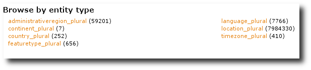
The main page of the Geoname application is illustrated in the screenshot below. It provides general information on the database, in particular the number of entities in the different classes:
- 7,984,330 locations.
- 59,201 administrative regions (e.g. regions, counties, departments...)
- 7,766 languages.
- 656 features (e.g. types of location).
- 410 time zones.
- 252 countries.
- 7 continents.
Simple query
We will first illustrate the possibilites of CubicWeb with the simple query that we have detailed before (that could be directly pasted in the url...):
Any X LIMIT 10 WHERE X is Location, X population > 1000000,
    X country C, C name "France"
We obtain the following page:
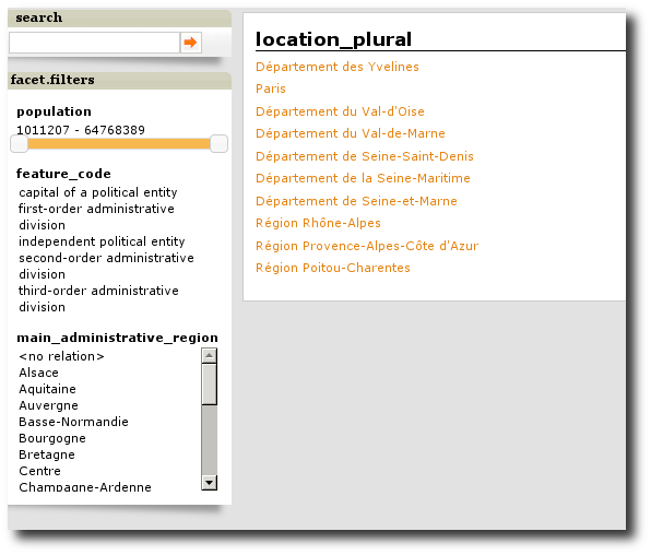
This is the standard view of CubicWeb for displaying results. We can see (right box) that we obtain 10 locations that are indeed located in France, with a population of more than 1,000,000 inhabitants. The left box shows the search panel that could be used to launch queries, and the facet filters that may be used for filtering results, e.g. we may ask to keep only results with a population greater than 4,767,709 inhabitants within the previous results:
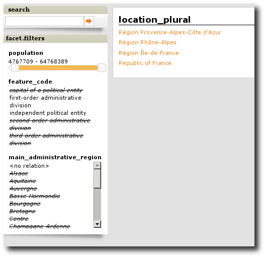
and we obtain now only 4 results. We can also notice that the facets are linked: by restricting the result set using the population facet, the other facets also restricted their possibilities.
Simple query (but with more information !)
Let's say that we now want more information about the results that we have obtained previously (for example the exact population, the elevation and the name). This is really simple ! We just have to ask within the RQL query what we want (of course, the names N, P, E of the variables could be almost anything...):
Any N, P, E LIMIT 10 WHERE X is Location,
    X population P, X population > 1000000,
    X elevation E, X name N, X country C, C name "France"
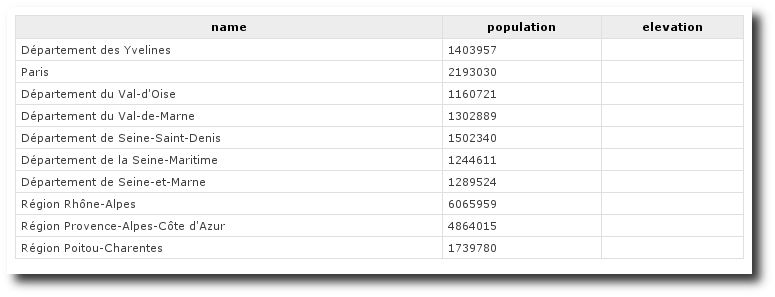
The empty column for the elevation simply means that we don't have any information about elevation.
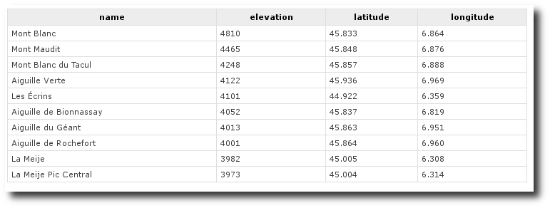
Anyway, we can see that fetching particular information could not be simpler! Indeed, with more complex queries, we can access countless information from the Geonames database:
Any N,E,LA,LO ORDERBY E DESC LIMIT 10  WHERE X is Location,
      X latitude LA, X longitude LO,
      X elevation E, NOT X elevation NULL, X name N,
      X country C, C name "France"
which means:
Give me the 10 highest locations (the 10 first when sorting by decreasing elevation) with their name, elevation, latitude and longitude that are in a country named "France"
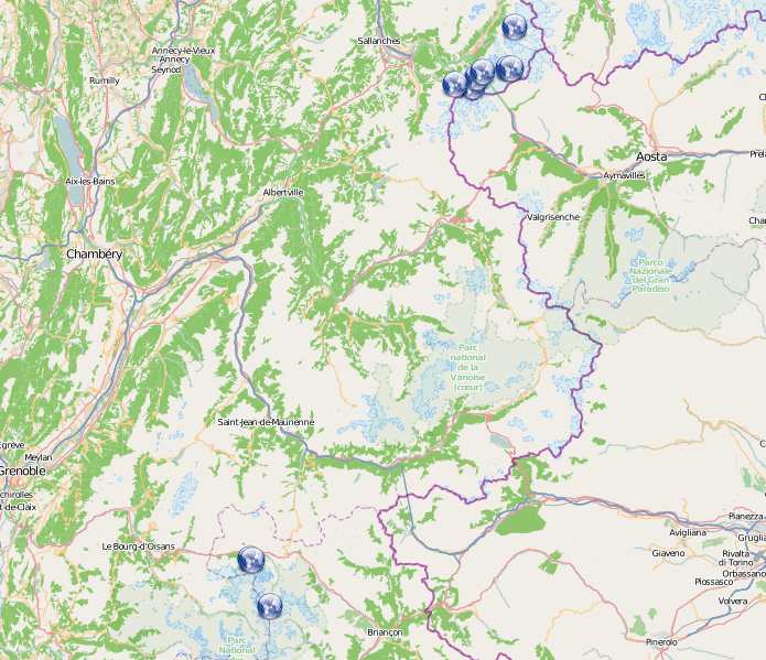
We can now use another view on the same request, e.g. on a map (view mapstraction.map):
Any X ORDERBY E DESC LIMIT 10  WHERE X is Location,
       X latitude LA, X longitude LO, X elevation E,
       NOT X elevation NULL, X country C, C name "France"
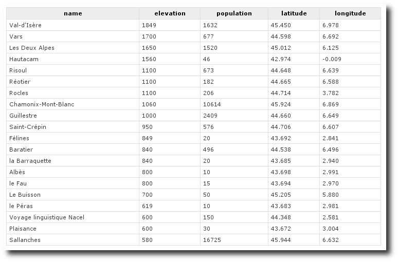
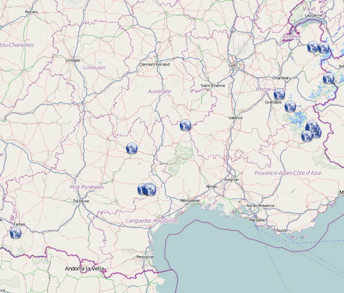
And now, we can add the fact that we want more results (20), and that the location should have a non-null population:
Any N, E, P, LA, LO ORDERBY E DESC LIMIT 20  WHERE X is Location,
       X latitude LA, X longitude LO,
       X elevation E, NOT X elevation NULL, X population P,
       X population > 0, X name N, X country C, C name "France"
... and on a map ...
Conclusion
In this blog, we have seen how CubicWeb could be used to store and query complex data, while providing (among other...) Web-based views for data vizualisation. It allows the user to directly query data within the URL and may be used to interact with and explore the data in depth. In a next blog, we will give more complex queries to show the full possibilities of the system.
